ST_GraphAnalysis

Signatures

Creates two tables:
    INPUT_EDGES_NODE_CENT[NODE_ID, BETWEENNESS, CLOSENESS]
    INPUT_EDGES_EDGE_CENT[EDGE_ID, BETWEENNESS]
ST_GraphAnalysis('INPUT_EDGES', 'o[ - eo]'[, 'w']);

Description

Uses Brande’s betweenness centrality algorithm to calculate closeness and betweenness centrality for vertices and betweenness centrality for edges.

Let \(d(s, t)\) denote the distance from \(s \in V\) to \(t \in V\), i.e., the minimum length of all paths connecting \(s\) to \(t\). We have \(d(s, s) = 0\) for all \(s \in V\).

Let \(\sigma_{st}\) denote the number of shortest paths from \(s \in V\) to \(t \in V\) and set \(\sigma_{ss}=1\) by convention.

Let \(\sigma_{st}(v)\) denote the number of shortest paths from \(s\) to \(t\) containing \(v \in V\).

We have the following definitions for vertices:

Closeness centrality (1)

(1)\[ C_C(v) = \left(\sum_{t \in V} d(v, t)\right)^{-1} \]

Betweenness centrality (2)

(2)\[ C_B(v) = \sum_{s \neq t \neq v \in V} \frac{\sigma_{st}(v)}{\sigma_{st}} \]

Betweenness centrality for edges is defined similarly.

A high closeness centrality score indicates that a vertex can reach other vertices on relatively short paths; a high betweenness centrality score indicates that a vertex lies on a relatively high number of shortest paths.

Note

All centrality scores are normalized

But this normalization depends on the graph being connected. Use ST_ConnectedComponents to make sure you’re calling ST_GraphAnalysis on a single (strongly) connected component

Warning

A few caveats

Results will not be accurate if the graph:

contains “duplicate” edges (having the same source, destination and weight)
is disconnected. If all closeness centrality scores are zero, this is why.

Though Brande’s algorithm is much faster than a naïve approach, it still requires an augmented version of Dijkstra’s algorithm to be run starting from each vertex. Thus, calculation times can be rather long for larger graphs.

Input parameters

Variable	Meaning
`INPUT_EDGES`	Table containing integer columns `EDGE_ID`, `START_NODE` and `END_NODE`; and optionally a weight column `w` (if the graph is weighted) and/or an edge orientation column `eo` (required if global orientation is not `undirected`)
`o`	Global orientation string: `directed`, `reversed` or `undirected`
`eo`	Edge orientation column name indicating individual edge orientations: `1` (directed), `-1` (reversed) or `0` (undirected); required if global orientation is `directed` or `reversed`
`w`	Edge weights column name

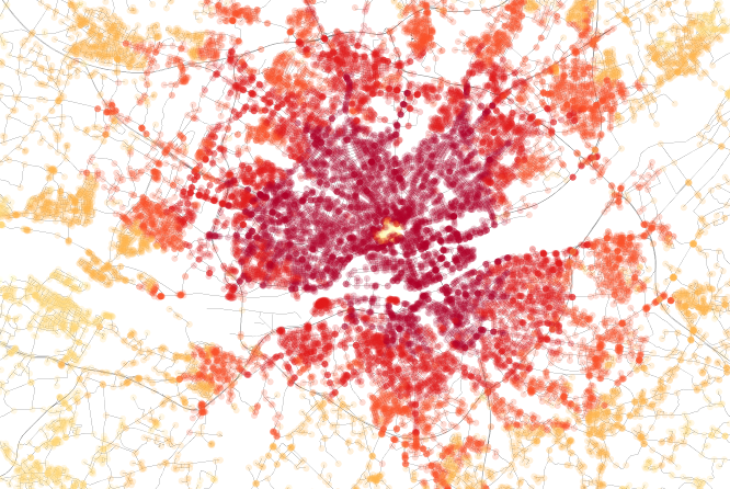
Screenshots

Closeness centrality of Nantes, France. Notice the limited traffic zone in the center.

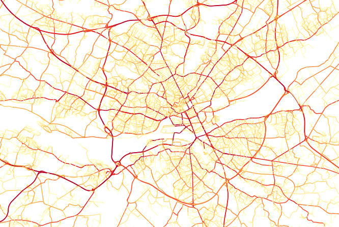
Edge betweenness centrality of Nantes, France. Notice how the beltway and bridges really stand out.

Examples

We will do graph analysis on the largest strongly connected component of the directed weighted graph examined in ST_ShortestPath examples, illustrated below

SELECT * FROM EDGES_EO_W_SCC;

EDGE_ID	START_NODE	END_NODE	WEIGHT	EDGE_ORIENTATION
1	1	2	10.0	1
2	2	4	1.0	-1
3	2	3	2.0	1
4	3	2	3.0	1
5	1	3	5.0	1
6	3	4	9.0	1
7	3	5	2.0	1
8	4	5	4.0	1
9	5	4	6.0	1
10	5	1	7.0	0

Do the graph analysis

CALL ST_GraphAnalysis('EDGES_EO_W_SCC',
    'directed - EDGE_ORIENTATION', 'WEIGHT');
-- The results for nodes:
SELECT * FROM EDGES_EO_W_SCC_NODE_CENT;

NODE_ID	BETWEENNESS	CLOSENESS
1	0.0	0.12121212121212122
2	0.3333333333333333	0.14814814814814814
3	0.8333333333333334	0.18181818181818182
4	0.3333333333333333	0.21052631578947367
5	1.0	0.13793103448275862

We use linear interpolation from red (0) to blue (1) to illustrate node betweenness

SELECT NODE_ID,
       BETWEENNESS,
       CAST(255*(1-BETWEENNESS) AS INT) RED,
       CAST(255*BETWEENNESS AS INT) BLUE
    FROM EDGES_EO_W_SCC_NODE_CENT
    ORDER BY BETWEENNESS DESC;

NODE_ID	BETWEENNESS	RED	BLUE
5	1.0	0	255
3	0.8333333333333334	42	213
4	0.3333333333333333	170	85
2	0.3333333333333333	170	85
1	0.0	255	0

We use linear interpolation from red (0) to blue (1) to illustrate closeness

SELECT NODE_ID,
       CLOSENESS,
       CLOSE_INTERP,
       CAST(255*(1-CLOSE_INTERP) AS INT) RED,
       CAST(255*CLOSE_INTERP AS INT) BLUE
   FROM (SELECT NODE_ID,
                CLOSENESS,
                (CLOSENESS - (SELECT MIN(CLOSENESS)
                                FROM EDGES_EO_W_SCC_NODE_CENT)) /
                ((SELECT MAX(CLOSENESS)
                    FROM EDGES_EO_W_SCC_NODE_CENT) -
                 (SELECT MIN(CLOSENESS)
                    FROM EDGES_EO_W_SCC_NODE_CENT))
                AS CLOSE_INTERP
         FROM EDGES_EO_W_SCC_NODE_CENT)
    ORDER BY CLOSENESS DESC;

NODE_ID	CLOSENESS	CLOSE_INTERP	RED	BLUE
4	0.21052631578947367	1.0	0	255
3	0.18181818181818182	0.6785714285714287	82	173
2	0.14814814814814814	0.3015873015873015	178	77
5	0.13793103448275862	0.18719211822660095	207	48
1	0.12121212121212122	0.0	255	0

The results for edges

SELECT * FROM EDGES_EO_W_SCC_EDGE_CENT ORDER BY BETWEENNESS DESC;

EDGE_ID	BETWEENNESS
7	1.0
9	0.8571428571428571
3	0.8571428571428571
10	0.5714285714285714
2	0.5714285714285714
5	0.42857142857142855
4	0.2857142857142857
8	0.2857142857142857
-10	0.14285714285714285
1	0.0
6	0.0

We use linear interpolation from red (0) to blue (1) to illustrate node betweenness.

SELECT EDGE_ID,
       BETWEENNESS,
       CAST(255*(1-BETWEENNESS) AS INT) RED,
       CAST(255*BETWEENNESS AS INT) BLUE
    FROM EDGES_EO_W_SCC_EDGE_CENT
    ORDER BY BETWEENNESS DESC;

EDGE_ID	BETWEENNESS	RED	BLUE
7	1.0	0	255
3	0.8571428571428571	36	219
9	0.8571428571428571	36	219
2	0.5714285714285714	109	146
10	0.5714285714285714	109	146
5	0.42857142857142855	146	109
4	0.2857142857142857	182	73
8	0.2857142857142857	182	73
-10	0.14285714285714285	219	36
1	0.0	255	0
6	0.0	255	0

Exercises

Use ST_ShortestPathTree to calculate the shortest path trees for nodes 1 through 5. Then use the definition of node betweenness to calculate betweenness by hand and verify the results above.
Make use of ST_ShortestPath to write a script that calculates node betweenness automatically without using ST_GraphAnalysis. Make sure you get the same results as above.
Repeat exercise 2 using ST_ShortestPathLength to verify node closeness.